Q1 (a) Explain the nature of managerial economics and discuss its relevance in modern business decision-making.
(~300 words)
Managerial Economics is a specialized branch of economics that deals with the application of economic principles and methods to business decision-making. It helps managers take rational and logical decisions under conditions of scarcity, risk, and uncertainty. While traditional economics focuses on theory, managerial economics focuses on practical problem solving.
Nature of Managerial Economics
Firstly, managerial economics is micro-economic in nature because it studies individual business units such as firms, industries, and consumers rather than the entire economy. It focuses on issues like demand analysis, pricing, production, cost control, and profit planning.
Secondly, it is normative, meaning it prescribes what managers should do to achieve objectives like profit maximization or cost minimization. It provides guidelines for decision-making rather than merely describing economic behavior.
Thirdly, managerial economics is pragmatic and applied. It combines theoretical concepts such as marginal analysis, elasticity, opportunity cost, and forecasting with real-world business situations. It helps managers convert abstract theories into workable solutions.
Fourthly, it considers risk and uncertainty. Business decisions are taken with incomplete information about future demand, costs, competition, and government policies. Managerial economics uses tools like probability, forecasting, and decision theory to reduce uncertainty.
Relevance in Modern Business Decision-Making
In today’s competitive business environment, managerial economics is highly relevant. It helps managers in demand forecasting, which ensures proper production planning. It aids in pricing decisions by studying elasticity of demand and market structures. Cost analysis helps firms control expenses and determine the optimum level of output.
Managerial economics is also useful in profit planning, capital budgeting, resource allocation, and strategic planning. For example, before launching a new product, a firm uses demand analysis, cost analysis, and opportunity cost principles. Thus, managerial economics enables managers to take scientific, informed, and efficient decisions, improving business performance and profitability.
Q1 (b) Explain the Law of Diminishing Marginal Utility (DMU) with suitable example.
(~300 words)
The Law of Diminishing Marginal Utility states that as a consumer consumes more and more units of a commodity, the additional satisfaction (marginal utility) obtained from each successive unit goes on decreasing, provided consumption of other goods remains constant.
Marginal utility refers to the extra satisfaction derived from consuming one additional unit of a good. According to this law, the first unit of a commodity gives the highest satisfaction, and each subsequent unit gives less satisfaction than the previous one. After a certain point, marginal utility may become zero or even negative.
Explanation of the Law
Human wants are limited. When a consumer consumes a commodity continuously, the intensity of want decreases gradually. As a result, the satisfaction obtained from additional units falls. This law assumes rational behavior, constant tastes, and continuous consumption of identical units.
The law explains why consumers are willing to pay a higher price for the first unit and a lower price for additional units. It also forms the basis of the downward-sloping demand curve.
Example
Consider a person eating mangoes:
| Mangoes Consumed | Total Utility | Marginal Utility |
|---|---|---|
| 1st Mango | 30 | 30 |
| 2nd Mango | 50 | 20 |
| 3rd Mango | 60 | 10 |
| 4th Mango | 65 | 5 |
| 5th Mango | 65 | 0 |
| 6th Mango | 60 | –5 |
Here, marginal utility decreases with each mango. The 5th mango gives zero utility, and the 6th gives negative utility.
Importance
The Law of DMU helps explain:
- Consumer equilibrium
- Demand behavior
- Pricing policies
- Taxation principles
Thus, the Law of Diminishing Marginal Utility is a fundamental concept of consumer behavior and plays an important role in managerial economics.
Q2 (a) What is the Opportunity Cost Principle? Explain with a simple example.
(~300 words)
The Opportunity Cost Principle states that the real cost of choosing one alternative is the value of the next best alternative that is sacrificed. Since resources are scarce, every choice involves giving up something else.
Opportunity cost is not always a monetary cost. It may include income, time, comfort, or satisfaction forgone by choosing one option over another.
Explanation
When managers make decisions, they must consider not only the direct cost of an action but also what they are giving up. Ignoring opportunity cost may lead to incorrect or inefficient decisions. Opportunity cost helps in choosing the most profitable and efficient alternative.
Simple Examples
- Business Example
A firm has ₹5 lakh and two options:
- Invest in Project A earning ₹80,000
- Invest in Project B earning ₹60,000
If the firm chooses Project A, the opportunity cost is ₹60,000.
- Personal Example
If a student chooses MBA instead of a job offering ₹3 lakh per year, the opportunity cost of MBA is the salary forgone.
Importance in Managerial Decisions
Opportunity cost is useful in:
- Capital budgeting
- Make or buy decisions
- Resource allocation
- Time management
- Choosing among alternative projects
Managers use this principle to ensure that scarce resources are used in the best possible way. Hence, opportunity cost is a key concept in managerial economics and rational decision-making.
Q2 (b) Differentiate between Cardinal Utility and Ordinal Utility with examples.
(~300 words)
Utility refers to the satisfaction derived from consuming a good. There are two main approaches to measuring utility: Cardinal Utility and Ordinal Utility.
Cardinal Utility
Cardinal utility assumes that satisfaction can be measured numerically in imaginary units called utils. According to this approach, a consumer can quantify how much satisfaction he gets from a product.
Example:
An apple gives 20 utils and a banana gives 10 utils. Therefore, an apple gives double satisfaction compared to a banana.
This approach is based on the Law of Diminishing Marginal Utility and was proposed by early economists like Marshall.
Ordinal Utility
Ordinal utility states that satisfaction cannot be measured numerically, but consumers can rank their preferences. The consumer can say which product he prefers but not by how much.
Example:
A consumer prefers tea over coffee and coffee over juice, but cannot measure satisfaction in numbers.
This approach is based on Indifference Curve Analysis and is considered more realistic.
Differences
| Basis | Cardinal Utility | Ordinal Utility |
|---|---|---|
| Measurement | Numerical | Ranking |
| Utility unit | Utils | No units |
| Approach | Old | Modern |
| Realism | Less | More |
| Analysis | Marginal utility | Indifference curves |
Conclusion
Ordinal utility is preferred in modern economics because satisfaction cannot be measured in exact numbers in real life.
Q3 (a) What are the exceptions to the Law of Demand? Explain with examples.
(~300 words)
The Law of Demand states that, other things remaining constant, when the price of a commodity rises, the quantity demanded falls, and when the price falls, quantity demanded rises. This law shows an inverse relationship between price and demand. However, in real life, there are certain situations where this law does not apply. These situations are called exceptions to the Law of Demand.
One important exception is Giffen goods. These are inferior goods consumed mainly by poor people. When the price of such goods increases, demand also increases because people cannot afford better substitutes. For example, if the price of coarse grains like jowar or bajra increases, poor consumers may buy more of it and reduce consumption of costly food items.
Another exception is Veblen goods, which are luxury or status goods. For such goods, a higher price increases demand because it gives a sense of prestige. Examples include diamonds, luxury cars, branded watches, and expensive perfumes. People buy them not for utility but for social status.
Speculation is another exception. If consumers expect prices to rise further in the future, they may buy more even when prices are rising. For example, during a rise in gold prices, people may buy more gold expecting further price increases.
Ignorance or illusion of quality also acts as an exception. Sometimes consumers believe that higher price means better quality. For example, expensive medicines or branded clothes may be preferred over cheaper ones.
In emergency situations like war, famine, or pandemics, people buy essential goods regardless of price increases. During COVID-19, demand for masks and sanitizers increased even at high prices.
Thus, due to psychological, social, and economic reasons, the Law of Demand does not operate in all situations.
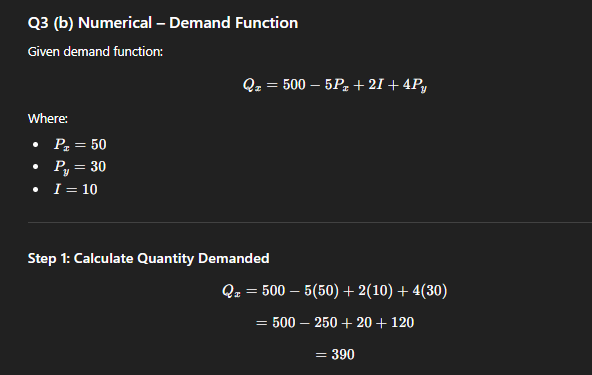
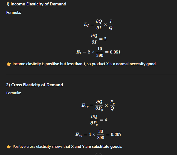
Q3 (b) Numerical – Demand Function
Q4 (a) State the Law of Supply and explain its application in managerial decision-making.
(~300 words)
The Law of Supply states that other things remaining constant, when the price of a commodity increases, the quantity supplied also increases, and when the price decreases, the quantity supplied decreases. Thus, price and quantity supplied have a direct relationship.
The main reason behind this law is the profit motive of producers. Higher prices mean higher profits, encouraging firms to produce and supply more. Lower prices reduce profits, so firms reduce supply.
Explanation with Example
Suppose the market price of rice increases from ₹40 to ₹60 per kg. Farmers will increase production by using more fertilizers, better seeds, and more land. If the price falls, they may reduce cultivation or shift to other crops.
Application in Managerial Decision-Making
The Law of Supply is very useful for managers in business decisions:
- Production Planning – Managers decide output levels based on expected price changes.
- Pricing Decisions – Understanding supply response helps firms adjust prices during shortages or surpluses.
- Capacity Utilization – At high prices, firms operate at full capacity to maximize profits.
- Inventory Management – Firms increase stock when prices are expected to rise.
- Market Entry Decisions – High prices attract new firms into the industry.
- Resource Allocation – Firms allocate resources to products with higher returns.
Thus, the Law of Supply helps managers plan production efficiently, maximize profits, and respond effectively to market conditions.
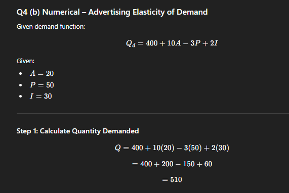
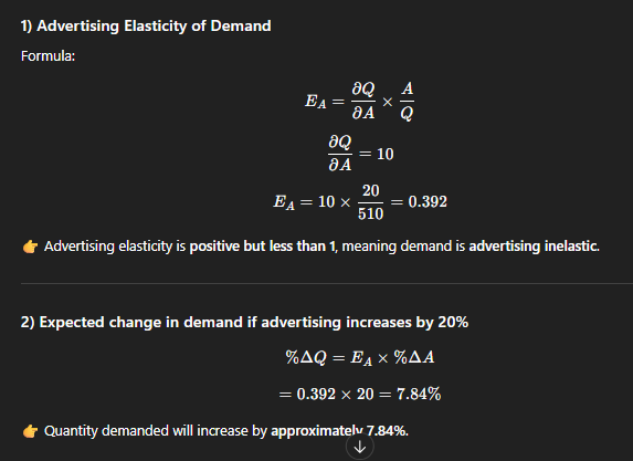
Q4 (b) Numerical – Advertising Elasticity of Demand
Q5 (a) Explain the Law of Diminishing Marginal Returns and provide an example of this phenomenon.
(~300 words)
The Law of Diminishing Marginal Returns is an important law of production in managerial economics. It states that when more and more units of a variable factor of production are combined with a fixed factor, the additional output (marginal product) obtained from each extra unit of the variable factor will eventually start declining, assuming technology remains unchanged.
This law operates in the short run, because at least one factor of production (such as land, machinery, or building) remains fixed, while others like labour or raw material can be varied. Initially, when additional units of labour are employed, productivity increases due to better division of labour, specialization, and efficient use of fixed resources. However, after a certain point, the fixed factor becomes a constraint. Too many workers start sharing the same machinery or space, leading to overcrowding, inefficiency, and poor coordination. As a result, marginal output declines.
Example
Consider a small agricultural farm with fixed land:
| Labour (Workers) | Total Output (kg) | Marginal Output |
|---|---|---|
| 1 | 10 | 10 |
| 2 | 25 | 15 |
| 3 | 45 | 20 |
| 4 | 60 | 15 |
| 5 | 70 | 10 |
| 6 | 75 | 5 |
After the third worker, marginal output starts falling. This shows diminishing marginal returns.
Importance
This law helps managers:
- Decide the optimum level of employment
- Avoid wastage of resources
- Control production costs
- Plan output efficiently
The Law of Diminishing Marginal Returns applies widely in agriculture, manufacturing units, factories, and service industries. Managers must understand this law to ensure efficient use of variable factors and to maximize productivity and profits.
Q5 (b) Numerical – MRTS
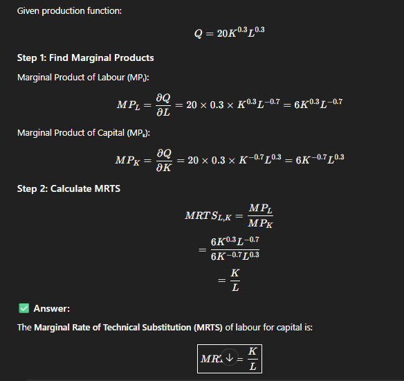
Q6 (a) Define Isoquants. Explain the different types of isoquants and discuss their properties.
(~300 words)
An isoquant is a curve that represents all possible combinations of two inputs, usually labour and capital, that produce the same level of output. Each point on an isoquant shows a technically efficient method of producing a given quantity of output. Isoquants are similar to indifference curves in consumer theory, but they relate to production instead of satisfaction.
Types of Isoquants
- Linear Isoquant
This shows perfect substitution between labour and capital. One input can completely replace the other at a constant rate. - Right-Angle (L-shaped) Isoquant
This represents perfect complementarity between inputs. Labour and capital must be used in fixed proportions, such as one machine with one operator. - Convex Isoquant
This is the most realistic type. It shows diminishing MRTS, meaning as more labour is used, less capital can be replaced.
Properties of Isoquants
- Downward sloping: To keep output constant, an increase in labour requires a decrease in capital.
- Convex to the origin: Due to diminishing MRTS.
- Do not intersect: Intersection would imply same output level equals two different outputs.
- Higher isoquant = higher output.
- Isoquants never touch axes, because production requires both inputs.
Importance
Isoquants help firms in:
- Choosing the least-cost combination of inputs
- Understanding input substitution
- Production planning and cost minimization
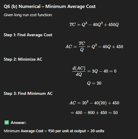
Q6 (b) Numerical – Minimum Average Cost
Q7 (a) Explain the features of Perfect Competition and describe price determination under perfect competition.
(~300 words)
Perfect competition is a market structure where a large number of buyers and sellers operate, and no single buyer or seller has the power to influence the market price. The price of the commodity is determined by the forces of demand and supply, and all firms are price takers.
Features of Perfect Competition
The first important feature is the large number of buyers and sellers. Each seller produces a very small portion of total market output, so no individual firm can affect price.
The second feature is homogeneous products. All firms sell identical products, so consumers do not prefer one seller over another. This leads to uniform pricing.
Thirdly, there is free entry and exit of firms. Firms can enter the market when profits exist and exit when losses occur. Due to this, firms earn only normal profit in the long run.
Another feature is perfect knowledge. Buyers and sellers have complete information about prices and quality. Hence, no seller can charge a higher price.
There is also perfect mobility of factors of production, allowing resources to move freely between industries.
Price Determination under Perfect Competition
Price is determined at the point where market demand equals market supply. This equilibrium price is accepted by all firms.
In the short run, firms may earn supernormal profits or incur losses depending on cost conditions. Firms produce where Marginal Revenue (MR) = Marginal Cost (MC).
In the long run, due to free entry and exit, supernormal profits disappear, and firms earn only normal profits.
Thus, perfect competition ensures efficient allocation of resources and fair pricing.
Q7 (b) Explain the barriers to entry in an oligopolistic market.
(~300 words)
Oligopoly is a market structure where a few large firms dominate the market. Entry of new firms is difficult due to several barriers to entry, which protect existing firms from competition.
One major barrier is high capital requirement. Oligopolistic industries like automobiles, steel, cement, and telecom require huge investment in plant, machinery, and technology. New firms often cannot afford this.
Another important barrier is economies of scale. Existing firms produce on a large scale and enjoy lower average costs. New firms producing on a smaller scale cannot compete with low prices.
Brand loyalty is also a strong barrier. Big firms spend heavily on advertising and build strong brand images. Consumers trust established brands, making it hard for new firms to attract customers.
Control over technology and patents restricts entry. Large firms invest heavily in research and development and may hold patents, preventing others from using similar technology.
Government policies and licensing can also restrict entry. Some industries require government approval, which limits competition.
Lastly, aggressive advertising and price wars by existing firms discourage new entrants, as they may not survive initial losses.
Thus, barriers to entry maintain oligopolistic power and limit competition.
Q8 (a) Compare monopoly and monopolistic competition with reference to pricing and output determination.
(~300 words)
Monopoly and monopolistic competition are two different market structures with distinct pricing and output policies.
In a monopoly, there is only one seller with no close substitutes. The monopolist is a price maker and has complete control over price and output. Entry of new firms is restricted due to legal, technical, or natural barriers.
Price and output under monopoly are determined where Marginal Revenue (MR) equals Marginal Cost (MC). After deciding output, the monopolist charges the price from the demand curve corresponding to that output. Price is usually higher and output lower compared to other market forms.
In monopolistic competition, there are many sellers selling differentiated products. Each firm has some control over price due to product differentiation, but this control is limited because close substitutes exist.
In the short run, firms may earn supernormal profits. In the long run, due to free entry and exit, firms earn only normal profits. Firms also operate with excess capacity.
Thus, monopoly results in higher prices and restricted output, while monopolistic competition provides product variety and moderate prices.
Q8 (b) Explain the role of monetary and fiscal policy in controlling recession.
(~300 words)
Recession is a phase of the business cycle characterized by falling output, income, employment, and demand. To control recession, governments use monetary policy and fiscal policy.
Role of Monetary Policy
Monetary policy is controlled by the central bank (RBI). During recession, the RBI adopts an expansionary monetary policy. It reduces interest rates, repo rate, and bank rate to make borrowing cheaper. This encourages businesses to invest and consumers to spend more.
The RBI also reduces Cash Reserve Ratio (CRR) and Statutory Liquidity Ratio (SLR), increasing the lending capacity of banks. Increased money supply boosts economic activity and employment.
Role of Fiscal Policy
Fiscal policy is implemented by the government. During recession, the government increases public expenditure on infrastructure, health, and education to generate employment.
It may also reduce taxes to increase disposable income, encouraging consumption. Subsidies and welfare schemes help boost demand among lower-income groups.
Conclusion
Monetary policy stimulates investment, while fiscal policy boosts consumption. Together, they increase aggregate demand and help the economy recover from recession.